Edit Exceptions of Pivot
In the ‘Set Exceptions’ page, you can apply unique colors to highlight values displayed in the pivot when certain exception criteria are met in the data. The visual impact of the highlighted cells enables users to pay attention to business data that does not fall within the normal range. You can highlight individual cells, sub totals, grand totals or combinations of these by assigning unique colors associated with exception conditions.
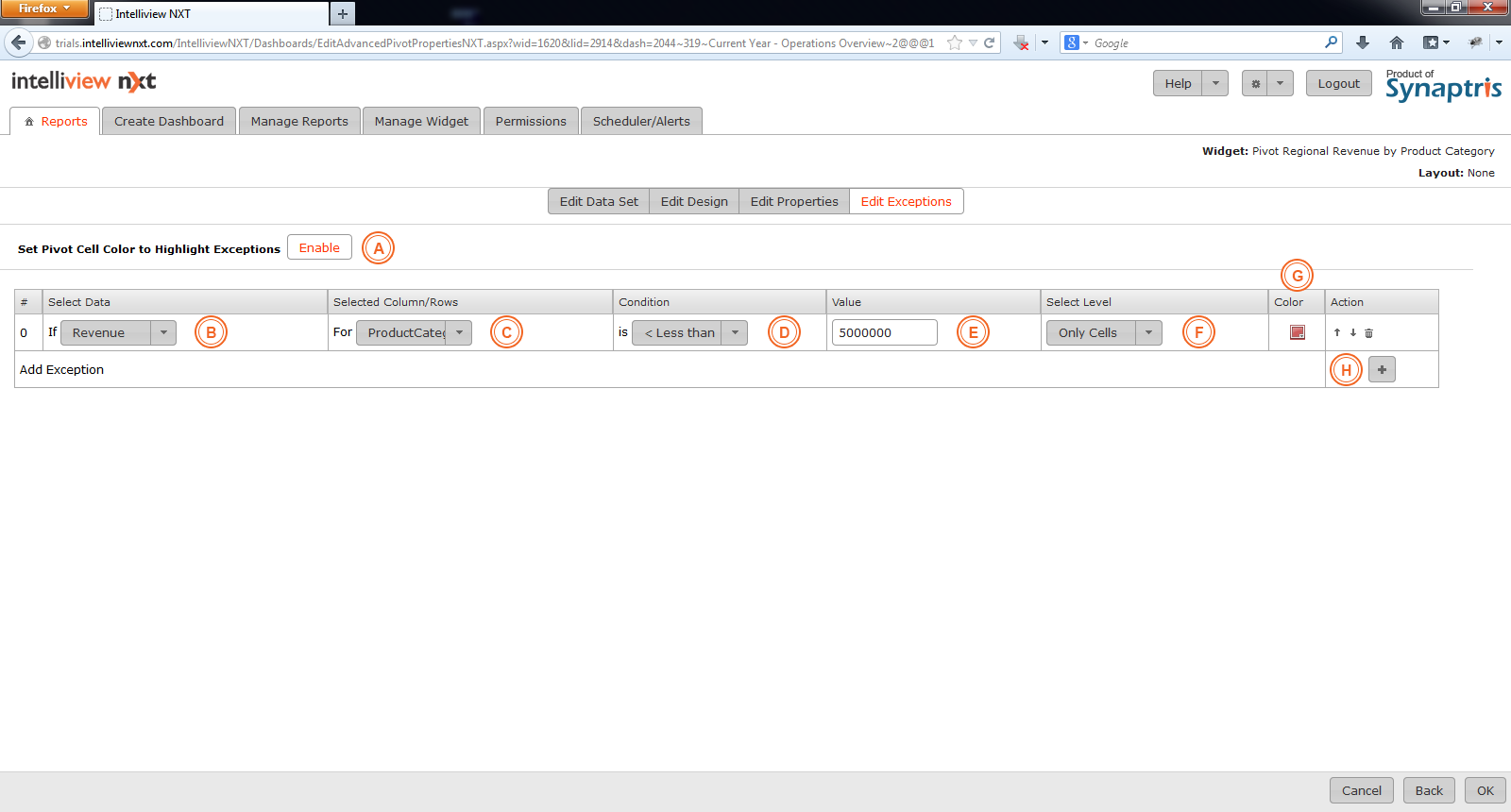
If you wish to highlight some of the data on your Pivot table by using color codes, you may do so by setting ‘exceptions’. In order to add an exception, the first step is to press the ‘Enable’ button on the Exceptions page.
Once the page is enabled, the next step is to press the + sign under the Action column. This will enable you to select the data and the rows and columns on which you wish to set exceptions. Select the conditions that the data must satisfy in order for the data cell to be color coded.
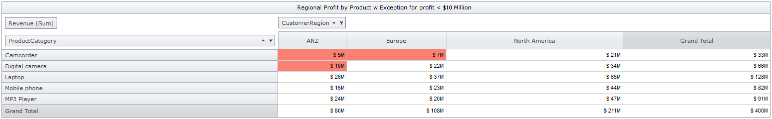
In the screenshot below, you can see that the exception is set to color cells where the ‘Revenue’ as a product category level is below $10 million to a light red color. Below that is a picture of the how the Pivot looks when the exception is applied.
You can add as many exceptions as you wish.
|

|
Exceptions are processed in a top to bottom sequence. If there is an overlap in conditions, the last condition in the list overrides the first condition in the list.
If you wish to disable exceptions, go to “Set Pivot Color to highlight Exceptions” and toggle the Enable button by clicking on it
The exception conditions defined in the Set Exceptions page can be used to setup Alert Monitoring under the Scheduler/Alerts menu. For more information, refer ‘Add Schedule for Alert Monitoring’.
|
|
A
|
The first step is to press ‘Enable’.
|
|
B
|
Press the + button to be able to add exceptions.
|
|
C
|
Choose the data column on which the condition is to be checked.
|
|
D
|
Pick the row or column of the table that you want highlighted.
|
|
E & F
|
Set the condition that must be satisfied for the cell to be highlighted in the selected color.
|
|
G
|
Select the specific area(s) of the Pivot you want highlighted when the Exception condition is met.
|
|
H
|
From the color wheel you may pick the color to be used when the Exception is triggered.
|
For the condition set above, the report will be color coded as seen below.

<< Edit Properties of Pivot | Edit Data Set of Table >>